I am writing these series of posts to challenge myself to enhance my skill in communciating machine learning and statistical concepts to others in an intuitive way
Bagging
Introduction
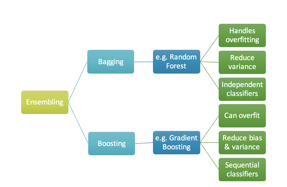
Bagging is an ensemble technique. In this method, instead of training just one tree, we train hundreds of trees and create an ensemble of the output at the end.
For each tree, instead of taking the entire data, we take only a few datapoints as a bagging sample.
Each tree is let to grow like any other normal tree. All the methods that are discussed in the “Decision trees” post are still applicable here.
At the end, all the hundreds of trees give different outputs and all these outputs are generally averaged to come up with the final class or prediction for a particular data point.
It is important to note that trees are not pruned in bagging methods. This is because if each tree overfits and has high variance, bagging will capture information from all these overfitted trees and results in a better output
Why bagging?
The main benefits of using this method is that it reduces the chances of overfitting and takes advantage of the weakness of different trees and create a single strong learner. If we have multiple trees that are uncorrelated, in other words, if they have high variance then the final ensembled output would have a higher accuracy as it is learning different values from different trees and will rightly learn different patterns present in the data.
Random Forest

Introduction
Random forest is one of the most famous bagging techniques in the machine learning community. The main difference between a normal bagging method and Random forest is that instead of considering all variables for a particular tree for the recursive split, we consider only a subset of variables. At each split, a random sample of m predictors is considered and is generally $\sqrt{P}$ where P is the total number of predictors. Split happens on of these m predictors. We can decide the size of subset but the variables for each tree are selected in a random manner.
All the trees present in a random forest can be tuned for hyper parameters that we discussed earlier. Even the numebr of variables that have to be selected for each tree can be fed into the hyper parameter method.
Key points to note:
- It creates a strong learner by combining the outputs from all the weak learners
- Random forest tends to run for longer times when the number of trees are more
- Size of tree and number of trees can be decided using k fold cross validation techniques
- If there is strong predictor in one tree, most of the trees will use this as a first split resulting in similar trees and correlated outputs. Average of correlated outputs will not lead to much reduction in variance. So it is preferable have weak predictors and use random forests to predict the output.
- Random forest will not overfit even with the increase in sample size (B)
- Variable importance measures plto gives the importance of all the variables after generating the ensemble output from all the trees.
- For classification tasks, majority vote is considered while making the final class selection
All trees present in a random forest can be tuned for hyper parameters that we discussed earlier.
Implementation in Python:
def random_forest(X,y):

    # Creating the train and test split
    from sklearn.model_selection import train_test_split
    X_train_m, X_val_m, y_train_m, y_val_m = train_test_split(X, y, test_size=0.3, random_state=1)

    from sklearn.ensemble import RandomForestClassifier
    from sklearn.model_selection import GridSearchCV
    from sklearn.metrics import confusion_matrix
    from sklearn.metrics import accuracy_score
    model = RandomForestClassifier(n_estimators = 250,max_features = None).fit(X_train_m, y_train_m)
#     grid_params = {'criterion': ['gini'], 'max_features' : [None], 'n_estimators': [300]}
#     para_search = GridSearchCV(model, grid_params, scoring = 'accuracy', cv = 5).fit(X_train_m, y_train_m)
#     best_model = para_search.best_estimator_
    labels_r = model.predict(X_val_m)

    train_mse = metrics.mean_squared_error(model.predict(X_train_m), y_train_m)
    test_mse = metrics.mean_squared_error(labels_r, y_val_m)
    print(train_mse)
    print(test_mse)
    print ('Accuracy using Random Forest:',accuracy_score(y_val_m, labels_r))
    mat_r = confusion_matrix(y_val_m, labels_r)
    print(mat_r)
    return model
For the entire code, refer to this notebook
Implementation in R:
# Random Forest
rf_model <- randomForest(class_labels_train ~ .,
                         data = X_train,
                         ntree = 1000)
author_predict <- predict(rf_model, X_test_pc, type = "response")
answer <- as.data.frame(table(author_predict, class_labels_test))
answer$correct <- ifelse(answer$author_predict==answer$class_labels_test, 1, 0)

answer_rf = answer %>% group_by(correct) %>% summarise("Correct" = sum(Freq))

rf_accuracy <- sum(answer$Freq[answer$correct==1])*100/sum(answer$Freq)

print(paste0("Accuracy is ", rf_accuracy))
For the entire code, refer to this notebook
That’s all folks! See you in the next article.
Happy learning!